💻 AI predictions in an online store - 01

This post is focused on building and training a machine learning model to predict whether a given instance is likely to accept third-party advertising. The dataset is loaded from a CSV file, and various preprocessing steps are applied before creating, training, and evaluating the model.
Import Required Libraries
The necessary libraries are imported, including TensorFlow for machine learning tasks, Pandas for data manipulation, and other utilities. TensorBoard logs are configured to visualize the model training progress.
# Suppress tensorflow optimization warnings
import os
os.environ['TF_CPP_MIN_LOG_LEVEL'] = '3'  # or '2' to also hide INFO messages

import tensorflow as tf
Load Dataset
The dataset is loaded from a CSV file named ‘dataset.csv’ using Pandas. The dataset is then copied to ensure the original data remains intact. For demonstration purposes, the dataset is truncated to the first one million rows.
import pandas as pd

raw_dataset = pd.read_csv('dataset.csv')
raw_dataset_copy = raw_dataset.copy()

# strip dataset to n values
raw_dataset_copy = raw_dataset_copy[:1000000]
Split Dataset
The dataset is split into training, validation, and test subsets using the train_test_split function from scikit-learn. The target variable ‘accept_third_party_advertising’ is separated from the input features.
from sklearn.model_selection import train_test_split
import numpy as np

x_raw = raw_dataset_copy
y_raw = x_raw.pop('accept_third_party_advertising')

x_train, x_temp, y_train, y_temp = train_test_split(x_raw, y_raw, test_size=0.2, random_state=24)
x_val, x_test, y_val, y_test = train_test_split(x_temp, y_temp, test_size=0.5, random_state=24)
Normalize Data
Data normalization is performed using TensorFlow’s Normalization layer. The layer is adapted to the training set and applied to normalize the training, validation, and test sets.
# Normalize the data using TensorFlow's Normalization layer
normalize = tf.keras.layers.Normalization()
normalize.adapt(x_train)

# Apply normalization to the training set
x_train_normalized = normalize(x_train)

# Apply normalization to the validation set
x_val_normalized = normalize(x_val)

# Apply normalization to the test set
x_test_normalized = normalize(x_test)
Create Model
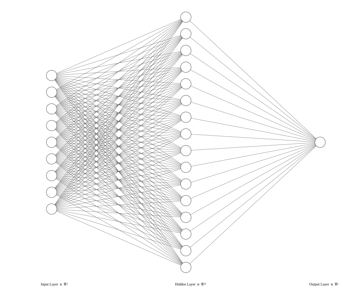
A simple neural network model is created using TensorFlow’s Sequential API. It consists of a normalization layer, a dense layer with 16 units and ReLU activation, and a final dense layer with a single unit and sigmoid activation, suitable for binary classification.
The model is compiled with the Adam optimizer, binary crossentropy loss function, and accuracy and precision metrics.
model = tf.keras.Sequential([
    normalize,
    tf.keras.layers.Dense(16, input_shape=(9,), activation='relu'),
    tf.keras.layers.Dense(1, activation='sigmoid') # [0, 1]
])

optimizer = tf.optimizers.Adam(learning_rate=0.001)

loss = tf.losses.BinaryCrossentropy()

model.compile(
    optimizer=optimizer,
    loss=loss,
    metrics=['accuracy', tf.keras.metrics.Precision()])

model.summary()
Train Model
The model is trained using the training set for two epochs. The training progress is monitored, and the results are visualized using matplotlib for accuracy and loss.
import matplotlib.pyplot as plt

history = model.fit(
    x=x_train,
    y=y_train,
    batch_size=None,
    epochs=10,
    callbacks=[tensorboard_callback],
    validation_data=(x_val, y_val))
Evaluate Model
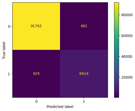
The model is evaluated on the test set, and the loss, accuracy, and precision are printed. Additionally, a confusion matrix is generated and displayed using scikit-learn’s confusion_matrix and ConfusionMatrixDisplay.
predicted = model.predict(x_test)

from sklearn.metrics import confusion_matrix, ConfusionMatrixDisplay

squeezed_pred = tf.squeeze(predicted)
filtered_pred = np.array([1 if x >= 0.5 else 0 for x in squeezed_pred])
actual = np.array(y_test)

conf_mat = confusion_matrix(actual, filtered_pred)
displ = ConfusionMatrixDisplay(confusion_matrix=conf_mat)

displ.plot()

In summary, this notebook demonstrates the end-to-end process of loading a dataset, preprocessing the data, creating a neural network model, training the model, and evaluating its performance using accuracy, precision metrics, and confusion matrix. The visualizations provided help in understanding how well the model performs on both training and test data.